pacman::p_load(ggrepel, patchwork,
               ggthemes, hrbrthemes,
               tidyverse, cluster,
               factoextra)
Installing package into 'C:/Users/kchan/AppData/Local/R/win-library/4.5'
(as 'lib' is unspecified)The objective of this project is to understand the behaviors behind customer transactions and how socio demographic factors such as age, income, and occupation affect customer transactions. By applying statistical correlation techniques, we aim to identify which personal attributes are the true drivers of financial activity within the Colombian fintech ecosystem.
Customer clustering techniques are used to group customers with similar financial behaviors and socio-demographic characteristics. By identifying distinct customer segments, the analysis provides insights into how different groups interact with fintech services, including their transaction patterns, savings behavior, and digital engagement levels.
The required R packages are loaded using the pacman::p_load() function, which automatically installs the packages if they are not already available and loads them into the working environment. These libraries support data manipulation, visualization, and clustering analysis required for the visual analytics application.
pacman::p_load(ggrepel, patchwork,
ggthemes, hrbrthemes,
tidyverse, cluster,
factoextra)Installing package into 'C:/Users/kchan/AppData/Local/R/win-library/4.5'
(as 'lib' is unspecified)The COFINFAD dataset consists of two files: a customer-level dataset containing 48,723 customer records and a transaction-level dataset containing over 3.1 million transaction entries. The customer dataset provides demographic, behavioral, engagement, and satisfaction attributes, while the transaction dataset stores transaction-level records including amount, date, and transaction type.
# Import datasets
# Import datasets
customer_data <- read_csv("data/customer_data.csv")
Rows: 48723 Columns: 54
── Column specification ────────────────────────────────────────────────────────
Delimiter: ","
chr (13): gender, location, income_bracket, occupation, education_level, ma...
dbl (29): customer_id, age, household_size, active_products, app_logins_fre...
lgl (7): savings_account, credit_card, personal_loan, investment_account, ...
date (5): first_tx, last_tx, last_survey_date, last_transaction_date, first...
ℹ Use `spec()` to retrieve the full column specification for this data.
ℹ Specify the column types or set `show_col_types = FALSE` to quiet this message.transactions_data <- read_csv("data/transactions_data.csv")Rows: 3159157 Columns: 4
── Column specification ────────────────────────────────────────────────────────
Delimiter: ","
chr (1): type
dbl (2): customer_id, amount
date (1): date
ℹ Use `spec()` to retrieve the full column specification for this data.
ℹ Specify the column types or set `show_col_types = FALSE` to quiet this message.# Preview datasets
head(customer_data)# A tibble: 6 × 54
customer_id age gender location income_bracket occupation education_level
<dbl> <dbl> <chr> <chr> <chr> <chr> <chr>
1 93716481 44 Male Pereira, R… Very High Engineer Master
2 49020929 44 Male Cali, Vall… Medium Construct… Bachelor
3 52690950 45 Male Barranquil… High Construct… Bachelor
4 23199751 45 Male Bogotá, Cu… High Electrici… High School
5 61997066 44 Female Bogotá, Cu… Medium Cleaner Bachelor
6 85721098 45 Female Bogotá, Cu… Medium Architect PhD
# ℹ 47 more variables: marital_status <chr>, household_size <dbl>,
# acquisition_channel <chr>, customer_segment <chr>, savings_account <lgl>,
# credit_card <lgl>, personal_loan <lgl>, investment_account <lgl>,
# insurance_product <lgl>, active_products <dbl>, app_logins_frequency <dbl>,
# feature_usage_diversity <dbl>, bill_payment_user <lgl>,
# auto_savings_enabled <lgl>, credit_utilization_ratio <dbl>,
# international_transactions <dbl>, failed_transactions <dbl>, …head(transactions_data)# A tibble: 6 × 4
customer_id date amount type
<dbl> <date> <dbl> <chr>
1 93716481 2023-11-23 1262800 Transfer
2 93716481 2023-01-05 928900 Withdrawal
3 93716481 2023-11-05 1683100 Payment
4 93716481 2023-04-14 4507350 Payment
5 93716481 2023-08-04 2096150 Payment
6 93716481 2023-03-29 2124050 Payment colnames(customer_data) [1] "customer_id" "age"
[3] "gender" "location"
[5] "income_bracket" "occupation"
[7] "education_level" "marital_status"
[9] "household_size" "acquisition_channel"
[11] "customer_segment" "savings_account"
[13] "credit_card" "personal_loan"
[15] "investment_account" "insurance_product"
[17] "active_products" "app_logins_frequency"
[19] "feature_usage_diversity" "bill_payment_user"
[21] "auto_savings_enabled" "credit_utilization_ratio"
[23] "international_transactions" "failed_transactions"
[25] "tx_count" "avg_tx_value"
[27] "total_tx_volume" "first_tx"
[29] "last_tx" "base_satisfaction"
[31] "tx_satisfaction" "product_satisfaction"
[33] "satisfaction_score" "nps_score"
[35] "last_survey_date" "support_tickets_count"
[37] "resolved_tickets_ratio" "app_store_rating"
[39] "feedback_sentiment" "feature_requests"
[41] "complaint_topics" "clv_segment"
[43] "monthly_transaction_count" "average_transaction_value"
[45] "total_transaction_volume" "transaction_frequency"
[47] "last_transaction_date" "preferred_transaction_type"
[49] "first_transaction_date" "weekend_transaction_ratio"
[51] "avg_daily_transactions" "customer_tenure"
[53] "churn_probability" "customer_lifetime_value" colnames(transactions_data)[1] "customer_id" "date" "amount" "type" The selected variables were chosen to represent multiple dimensions of customer behavior. Variables such as tx_count, avg_tx_value, monthly_transaction_count, and transaction_frequency capture transaction intensity, while active_products, app_logins_frequency, and feature_usage_diversity reflect platform engagement. satisfaction_score, nps_score, and churn_probability were included to account for customer sentiment and retention risk, and customer_lifetime_value was included to reflect long-term business value.
cluster_data <- customer_data %>%
select(
age,
active_products,
app_logins_frequency,
feature_usage_diversity,
tx_count,
avg_tx_value,
monthly_transaction_count,
transaction_frequency,
satisfaction_score,
nps_score,
churn_probability,
customer_lifetime_value
)The correlation heatmap was used to examine relationships between selected variables. Highly correlated variables were evaluated to avoid redundancy in clustering.
library(corrplot)corrplot 0.95 loadedcor_matrix <- cor(cluster_data, use = "complete.obs")
corrplot(cor_matrix,
method = "color",
type = "upper",
tl.cex = 0.7)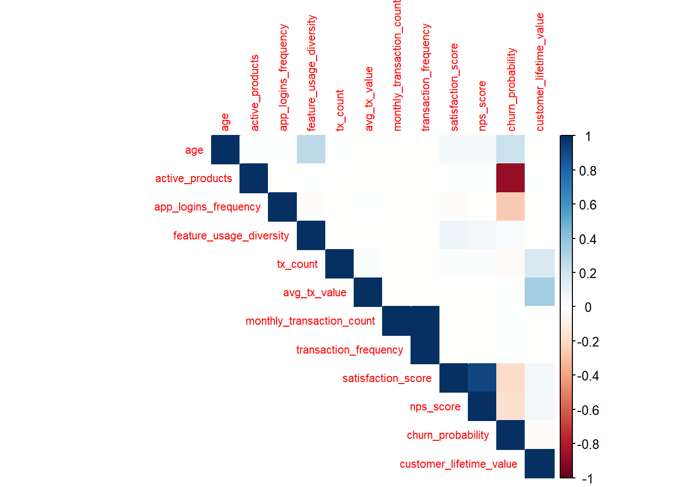
The heatmap indicates strong positive correlations among transaction-related variables such as transaction_frequency, monthly_transaction_count, and avg_tx_value, suggesting that customers who transact more frequently also tend to generate higher total financial activity. In contrast, engagement variables such as feature_usage_diversity and app_logins_frequency show moderate relationships with transaction metrics, indicating that behavioral engagement and financial value capture different dimensions of customer activity.
Before performing clustering, missing values were handled to ensure data quality and prevent errors during analysis. Observations containing missing values were removed to create a clean dataset for clustering.
cluster_data <- na.omit(cluster_data)Since the selected variables are measured on different scales (e.g., transaction volume, satisfaction scores, and login frequency), the data was standardized. Standardization ensures that all variables contribute equally to the clustering process.
cluster_scaled <- scale(cluster_data)K-means clustering was selected because the chosen variables are primarily continuous numeric measures that describe customer behavior, engagement, and financial activity. After standardization, K-means provides a simple and interpretable way to group customers based on similarity across these dimensions.
set.seed(123)

# take a sample for elbow method
cluster_sample <- as.data.frame(cluster_scaled) %>%
  slice_sample(n = 10000)

# compute WSS manually
wss <- numeric(10)

for (i in 1:10) {
  km <- kmeans(cluster_sample, centers = i, nstart = 10)
  wss[i] <- km$tot.withinss
}

# plot elbow curve
plot(1:10, wss, type = "b",
     xlab = "Number of Clusters",
     ylab = "Within-cluster Sum of Squares",
     main = "Elbow Method for Optimal Number of Clusters")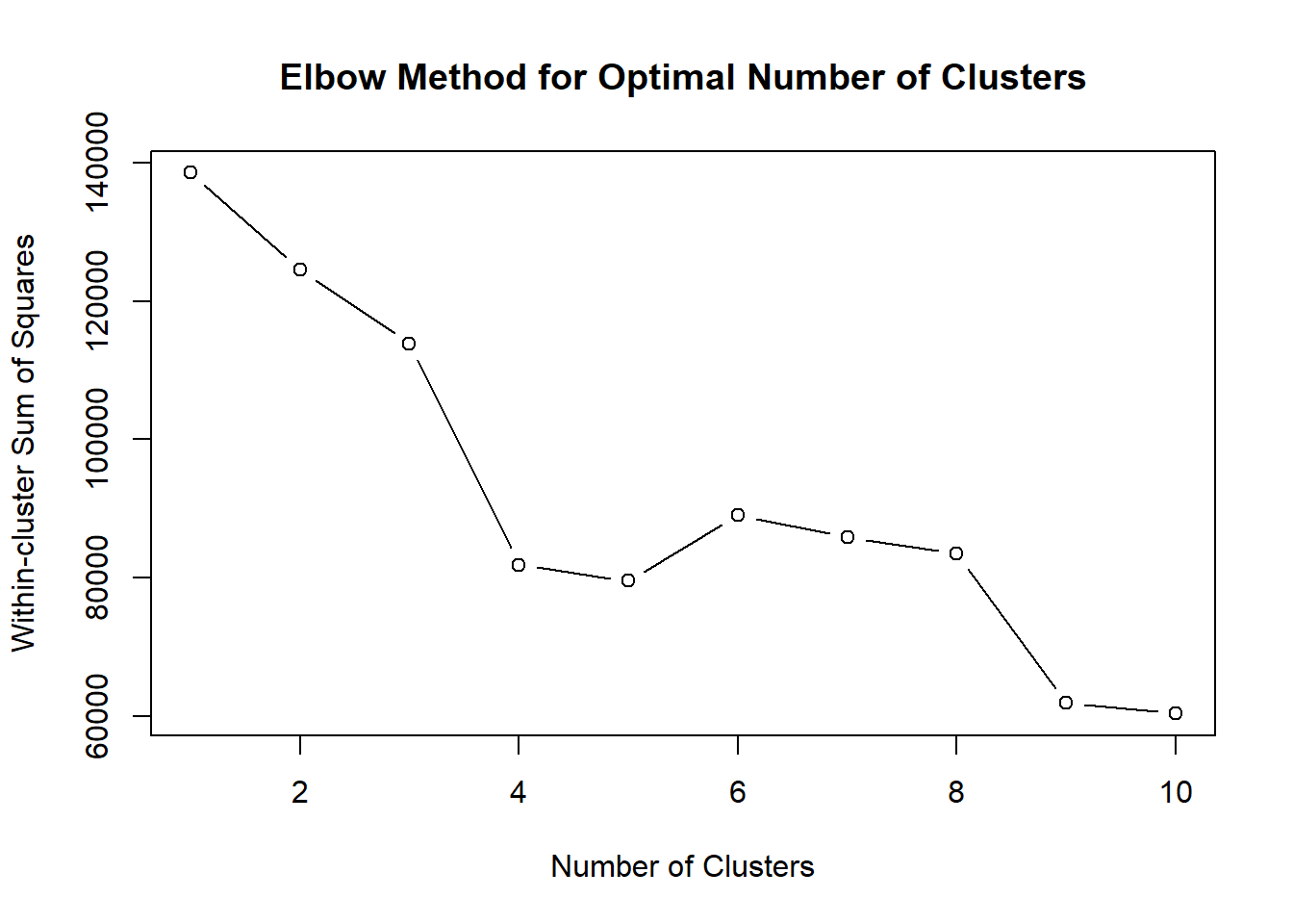
The elbow plot shows a sharp decrease in within-cluster sum of squares between k=1 and k=4, after which the improvement begins to diminish. This suggests that adding additional clusters beyond four provides limited reduction in within-cluster variance. Therefore, k = 4 appears to provide a good balance between model simplicity and cluster compactness.
sil_width <- numeric(9)

for (k in 2:10) {
  km <- kmeans(cluster_sample, centers = k, nstart = 10)
  ss <- silhouette(km$cluster, dist(cluster_sample))
  sil_width[k - 1] <- mean(ss[, 3])
}

plot(2:10, sil_width, type = "b",
     xlab = "Number of Clusters",
     ylab = "Average Silhouette Width",
     main = "Silhouette Analysis for Optimal Number of Clusters")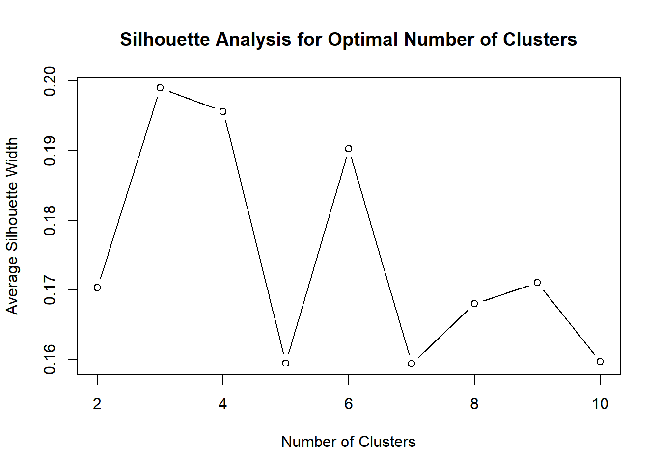
The silhouette analysis shows that the highest average silhouette width is achieved at 3 clusters, while 4 clusters also produces a relatively strong result. Since 4 clusters provides a more detailed and interpretable segmentation structure while maintaining acceptable cluster quality, it was selected for the final K-means model.
set.seed(123)
kmeans_model <- kmeans(cluster_scaled, centers = 4, nstart = 25)The final clustering model was estimated using K-means with 4 clusters and 25 random starts to improve stability and reduce the chance of converging to a poor local solution.
customer_data$cluster <- kmeans_model$clustertable(customer_data$cluster)
    1     2     3     4
4450 24263 9824 10186 ggplot(customer_data, aes(x = factor(cluster))) +
geom_bar(fill = "steelblue") +
labs(
title = "Customer Distribution by Cluster",
x = "Cluster",
y = "Number of Customers"
)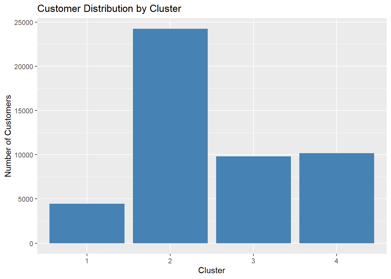
The distribution shows that Cluster 2 contains the largest number of customers, indicating that a dominant behavioral pattern exists among platform users. In contrast, Clusters 1, 3, and 4 represent smaller but still meaningful segments. This imbalance suggests that while most customers share similar behavioral characteristics, smaller groups exhibit distinct financial engagement patterns.
To better understand the separation between clusters, the clustering results were visualized using dimensionality reduction techniques. This visualization provides an overview of how customers are grouped based on their behavioral and financial characteristics.
fviz_cluster(kmeans_model,
             data = cluster_scaled,
             geom = "point",
             ellipse.type = "convex",
             show.clust.cent = TRUE)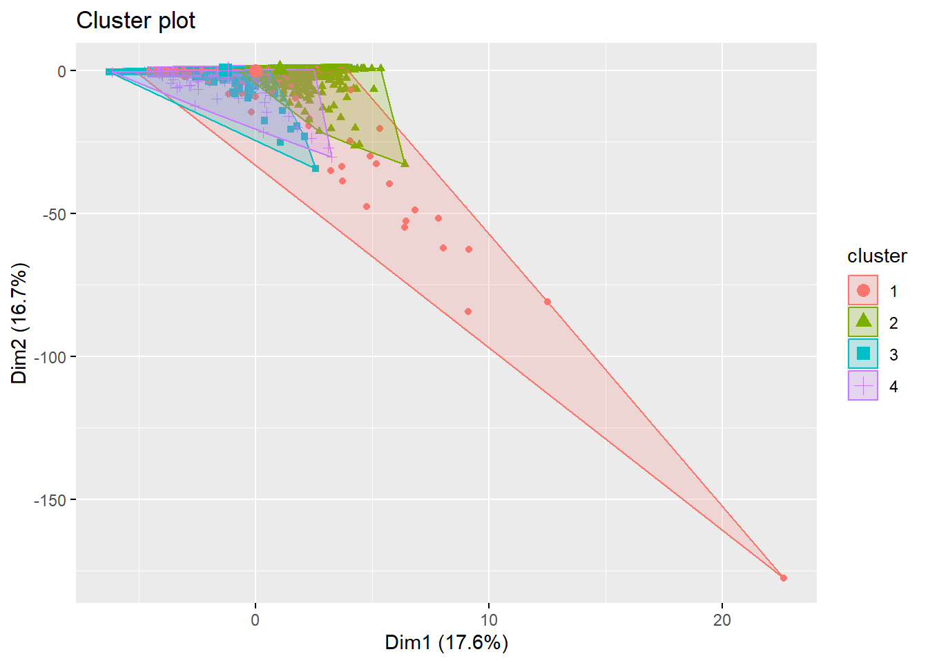
The cluster visualization based on the first two principal components shows partial separation among clusters, indicating that the segmentation captures meaningful differences in customer behavior. Although some overlap exists, distinct cluster regions can still be observed, suggesting that the clusters represent moderately differentiated customer groups. ### Variance Explained by Principal Components
pca_model <- prcomp(cluster_scaled)

fviz_eig(pca_model)
Warning in geom_bar(stat = "identity", fill = barfill, color = barcolor, :
Ignoring empty aesthetic: `width`.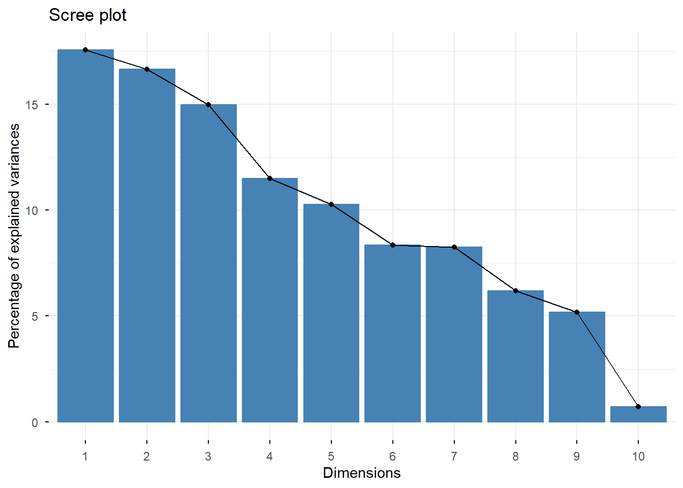
The scree plot indicates that the first few principal components explain a substantial proportion of the variance in the dataset. These components are therefore used to visualize the cluster structure in a reduced dimensional space.
Analyze Cluster Characteristics
To interpret the meaning of each cluster, the average values of key variables were calculated for each cluster. This allows us to identify behavioral patterns and characteristics that distinguish different customer segments.
cluster_summary <- customer_data %>%
  group_by(cluster) %>%
  summarise(
    avg_age = mean(age, na.rm = TRUE),
    avg_products = mean(active_products),
    avg_logins = mean(app_logins_frequency),
    avg_transactions = mean(tx_count),
    avg_tx_value = mean(avg_tx_value),
    avg_satisfaction = mean(satisfaction_score),
    avg_nps = mean(nps_score),
    avg_churn = mean(churn_probability),
    avg_clv = mean(customer_lifetime_value)
  )

cluster_summary
# A tibble: 4 × 10
cluster avg_age avg_products avg_logins avg_transactions avg_tx_value
<int> <dbl> <dbl> <dbl> <dbl> <dbl>
1 1 44.2 1.96 22.5 245. 13476030.
2 2 44.8 1.51 22.0 37.8 2475327.
3 3 45.9 1.75 21.9 64.7 2652231.
4 4 42.8 3.87 23.7 50.7 2710343.
# ℹ 4 more variables: avg_satisfaction <dbl>, avg_nps <dbl>, avg_churn <dbl>,
# avg_clv <dbl>The cluster summary shows meaningful differences across segments. Cluster 1 stands out for having the highest average transaction value and customer lifetime value, suggesting a high-value segment. Cluster 2 is the largest group but shows lower average transaction intensity and lower financial value, indicating a mainstream but less valuable segment. Cluster 4 stands out for having the highest number of active products and logins, suggesting a highly engaged digital segment. Cluster 3 appears to sit between these groups, with moderate engagement and transaction activity.
To better compare the characteristics of different clusters, key behavioral and financial variables were visualized across clusters. This helps highlight the differences between customer segments.
ggplot(customer_data, aes(x = factor(cluster), y = tx_count)) +
  geom_boxplot(fill = "orange") +
  labs(
    title = "Transaction Count by Cluster",
    x = "Cluster",
    y = "Transaction Count"
  )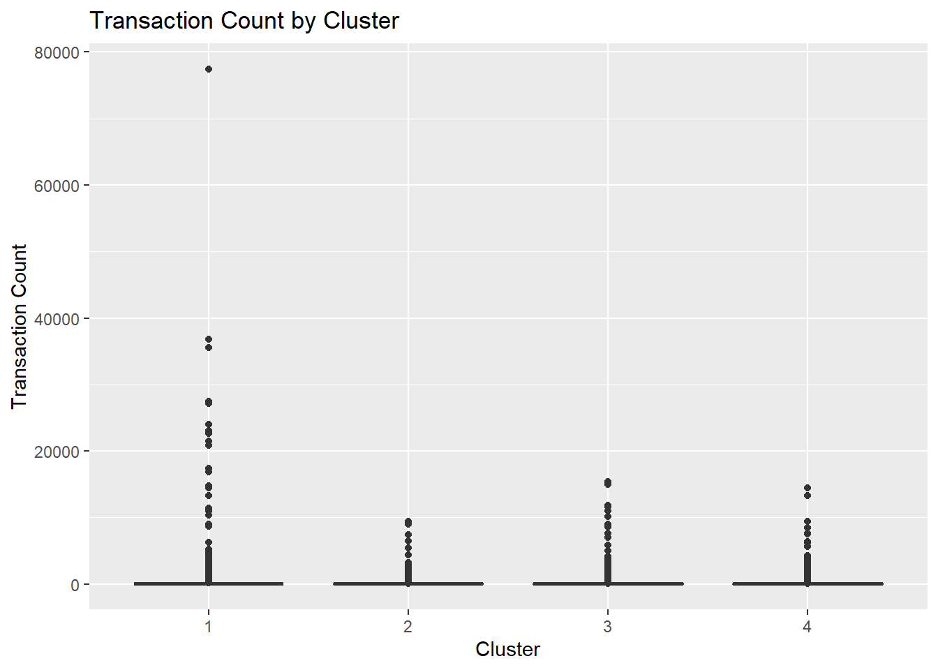
The clustering results reveal distinct customer segments within the fintech platform. For instance, some clusters represent highly active customers with frequent transactions and high customer lifetime value, while others represent lower engagement users with fewer financial activities and higher churn probability.
ggplot(customer_data, aes(x = factor(cluster), y = avg_tx_value)) +
  geom_boxplot(fill = "skyblue") +
  labs(
    title = "Average Transaction Value by Cluster",
    x = "Cluster",
    y = "Average Transaction Value"
  )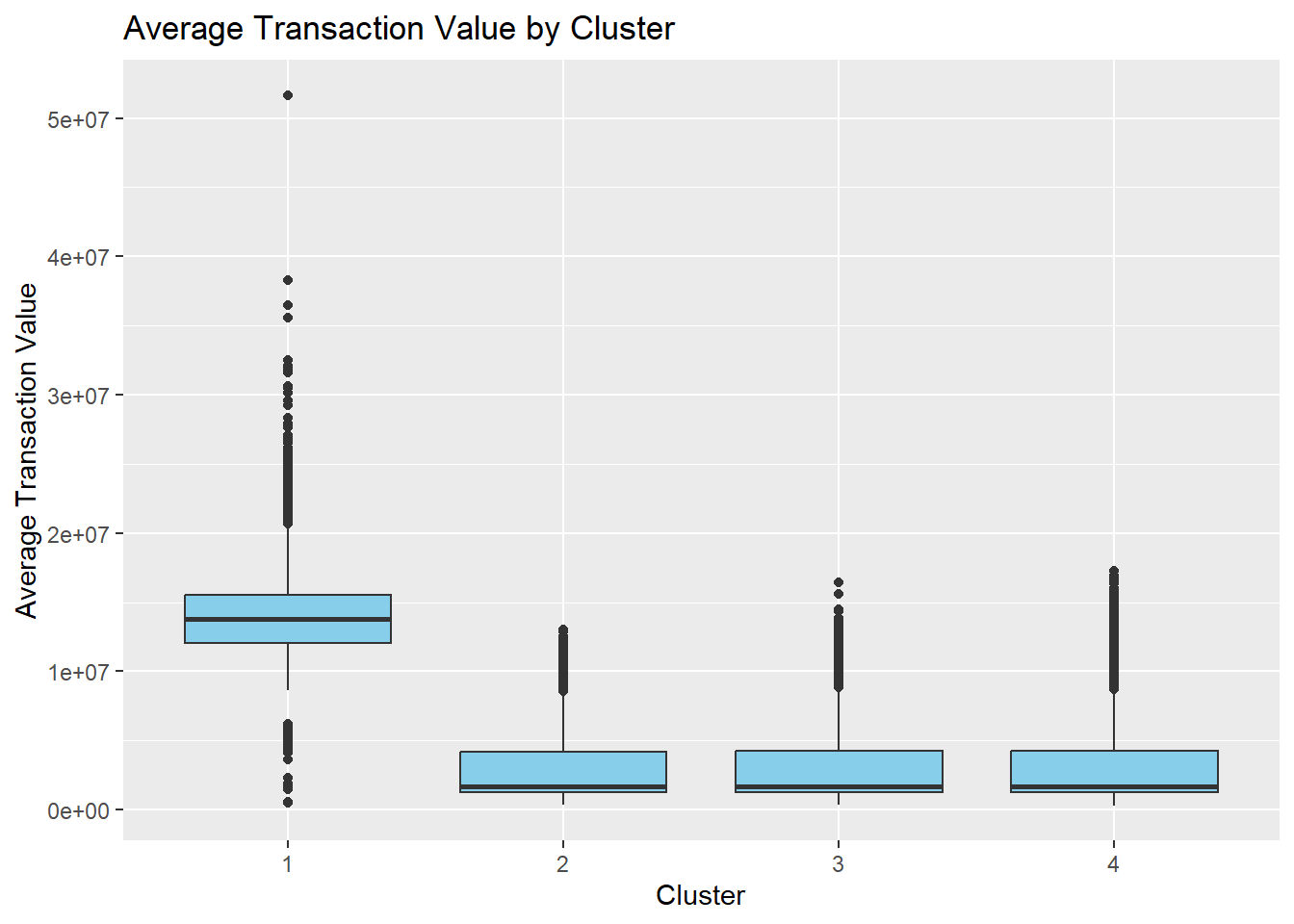
The profiling plots confirm that clusters differ not only in transaction count but also in financial value and engagement intensity. This suggests that the identified segments are behaviorally meaningful and can be used to distinguish high-value, low-activity, and digitally engaged customer groups.
library(tidyr)

cluster_profile_long <- cluster_summary %>%
  pivot_longer(-cluster, names_to = "metric", values_to = "value") %>%
  group_by(metric) %>%
  mutate(value_scaled = as.numeric(scale(value)))

ggplot(cluster_profile_long,
       aes(x = metric, y = value_scaled, color = factor(cluster), group = cluster)) +
  geom_line(linewidth = 1) +
  geom_point(size = 2) +
  theme_minimal() +
  labs(
    title = "Standardized Comparison of Cluster Characteristics",
    x = "Metric",
    y = "Standardized Value",
    color = "Cluster"
  ) +
  theme(axis.text.x = element_text(angle = 45, hjust = 1))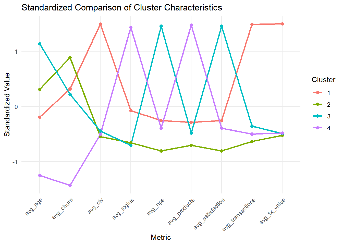
Because the metrics are measured on very different scales, the cluster comparison values were standardized before plotting. This makes it easier to compare relative differences across clusters without the chart being dominated by high-magnitude variables such as customer lifetime value.
ggplot(customer_data, aes(x = factor(cluster), fill = income_bracket)) +
  geom_bar(position = "fill") +
  labs(
    title = "Income Bracket Composition Across Clusters",
    x = "Cluster",
    y = "Proportion"
  )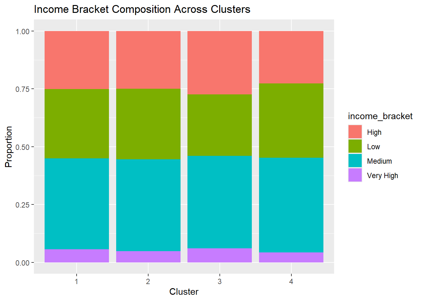
The income composition chart shows that the majority of customers across all clusters fall within the medium income bracket, with relatively smaller proportions in the low, high, and very high income categories. The distributions are broadly similar across clusters, suggesting that income level alone is not the primary factor driving the clustering structure. Instead, the clusters appear to be more strongly differentiated by behavioral and engagement-related variables, such as transaction activity, app usage, and product adoption.